Everything about Vehicle Simulation: 2017

Thursday, December 21, 2017

[Matlab] Animate a plot and Play a video

A plot can be animated along with x axis, and a video also can be played in Matlab.

Three basic techniques are used for creating animations.
1. Update the properties of a graphics object and display the updates on the screen. This is useful for creating animations when most of the graph remains the same.
2. Apply transforms to objects. This is useful when you want to operate on the position and orientation of a group of objects together.
3. Create a movie. Movies are useful if you have a complex animation that does not draw quickly in real time, or if you want to store an animation to replay it. Use the getframe and movie functions to create a movie.

Below are examples for animations.

1. Plot animation

%% Real time floating axis
h = animatedline;
% axis([0,12,-1,1]);
timestep = 0.1;
x = 0:timestep:12;%4*pi;
y = sin(x);
tic; % start timer
% h = animatedline(x,y,'Color','r','LineWidth',2);

for k = 1:length(x)
addpoints(h,x(k),y(k));
b=toc;% check timer
if k==1
timestep = 0;
else
if b < timestep % Calculated time is bigger than timer?
pause(timestep - b); % Then, pause until time = timer
drawnow % update
else
drawnow
end
end
%timestep;
timestep = timestep + 0.1;
end

2. Play a video

% Load a video file
video = 'C:\movie.avi';
% Read a file
v = VideoReader(video);
vWid = v.Width; vHei = v.Height;
% Frame per second
fps = get(v, 'FrameRate');
currAxes = axes;
v.CurrentTime = 0;% Specify the starting time [sec]
v.Duration % [sec] Unable to set ths property. Read-only property. Total play time
tic;
k=0;
while hasFrame(v)
vidFrame = readFrame(v);
ts = toc;
image(vidFrame, 'Parent', currAxes);% Display each frame
currAxes.Visible = 'off';
if ts <= k
pause(k-ts); % Wait until time = timer
end
k=k+1/fps; % Calculate time
end

Wednesday, December 20, 2017

[Matlab] Publish function (Create a report automatically)

It is often required to print a formatted report for results. Publish enables us to automatically create a report after simulation.
* For better report, see Matlab Report Generator
It supports html, doc, ppt, pdf, latex, and xml format as report, and the recommended format is html and pdf.

>> help publish

https://www.mathworks.com/help/matlab/matlab_prog/marking-up-matlab-comments-for-publishing.html

Monday, December 18, 2017

[Simulink] Moving average design without Signal Processing Toolbox

When designing a moving average filter in Simulink, it is normally not hard to create a model with basic Simulink blocks. However, in case of designing a moving average filter of 100 window size, it is not good idea to add 100 blocks of the Delay. So instead of using the Delay, we can use the block 'Matlab Function' where a moving average filter is coded.

* code

Wednesday, December 13, 2017

[Matlab] CANalyzer blf file to mat file conversion (Link)

https://jp.mathworks.com/matlabcentral/answers/342608-canalyzer-blf-file-to-mat-file-conversion

download

Monday, November 20, 2017

[Simulink] Lithium Battery Model, Simscape Language and Simulink Design Optimization

Sunday, November 19, 2017

[Simulink] Model Management

1. Using a Simulink Project with SVN
https://www.mathworks.com/help/simulink/examples/using-a-simulink-project-with-svn.html

2. Using a Simulink Project with Git
https://www.mathworks.com/help/simulink/examples/using-a-simulink-project-with-git.html

3. Simulink Example
https://www.mathworks.com/help/simulink/examples.html#d2e1680

Wednesday, November 8, 2017

[Modelica] Physical modeling language: Introduction & Useful link

Modelica is a non-proprietary, object-oriented, equation-based language to conveniently model complex physical systems containing, e.g., mechanical, electrical, electronic, hydraulic, thermal, control, electric power or process-oriented subcomponents.

Modelica Libraries with a large set of models are available. Especially, the open source Modelica Standard Library contains about 1600 model components and 1350 functions from many domains.

Modelica Simulation Environments are available commercially and free of charge, such as CATIA systems, Dymola, LMS AMESim, JModelica.org, MapleSim, OpenModelica, SCICOS, SimulationX, and Wolfram SystemModeler. Modelica models can be imported conveniently into Simulink uisng export features of Dymola MapleSim, and SimulationX.

https://www.modelica.org/

https://www.openmodelica.org/

http://fmi-standard.org/

http://book.xogeny.com/

Monday, November 6, 2017

[Matlab GUI] Resize the components such as axes, pushbutton, and so on on figure

There are two ways to resize components in figures when developing GUIs with GUIDE as below.

1. Menu Tools>GUI options>Resize behavior : Proportional
2. Menu Tools>GUI options>Resize behavior : Other (Use SizeChangedFcn)

Let's figure out two ways in details.
1. Menu Tools>GUI options>Resize behavior : Proportional
It is easy and simple to resize the components in figure with only selecting this option. However, the size is always changed proportional to the size of figure.
The units of all components are changed to 'normalized'.
Therefore, if you set the units of some components to other units which are not 'normalized', then the resize of those components is unavailable.

2. Menu Tools>GUI options>Resize behavior : Other (Use SizeChangedFcn)
If you select the resize behavior 'Other', then you have to create the SizeChangeFcn.

This function is easily added to the code by right-clicking on the GUIDE layout.

Example code
1. GUIDE layout

2. OpeningFcn function
% --- Executes just before resizeTest is made visible.
function resizeTest_OpeningFcn(hObject, eventdata, handles, varargin)
% This function has no output args, see OutputFcn.
% hObject handle to figure
% eventdata reserved - to be defined in a future version of MATLAB
% handles structure with handles and user data (see GUIDATA)
% varargin command line arguments to resizeTest (see VARARGIN)

% Choose default command line output for resizeTest
handles.output = hObject;

% Change the units of components
set(handles.pushbutton1,'Units','characters');
set(handles.uipanel1,'Units','characters');
set(handles.axes1,'Units','characters');
set(handles.figure1,'Units','characters');
% Get the initial position
fp = get(handles.figure1,'Position');
bp = get(handles.pushbutton1,'Position');
pp = get(handles.uipanel1,'Position');
ap = get(handles.axes1,'Position');

handles.fp = fp;
handles.bp = bp;
handles.pp = pp;
handles.ap= ap;
handles.yfromup = fp(4) - bp(2);assignin('base','yf',handles.yfromup);
% Update handles structure
guidata(hObject, handles);

3. resize function added by right-clicking

% --- Executes when figure1 is resized.
function figure1_SizeChangedFcn(hObject, eventdata, handles)
% hObject handle to figure1 (see GCBO)
% eventdata reserved - to be defined in a future version of MATLAB
% handles structure with handles and user data (see GUIDATA)

set(handles.pushbutton1,'Units','characters');
set(handles.uipanel1,'Units','characters');
set(handles.axes1,'Units','characters');
set(handles.figure1,'Units','characters');

figpos = get(handles.figure1,'Position');
buttonpos = get(handles.pushbutton1,'Position');
panelpos = get(handles.uipanel1,'Position');
axespos = get(handles.axes1,'Position');

% Set a push button position to fix the size and position
btopgab = handles.fp(4) - handles.bp(2);
buttonbottom = figpos(4) - btopgab;
set(handles.pushbutton1,'Position',[buttonpos(1) buttonbottom buttonpos(3) buttonpos(4)]);
% Set a uipanel position to fix the size and position
ptopgab = handles.fp(4) - handles.pp(2);
panelbottom = figpos(4) - ptopgab;
set(handles.uipanel1,'Position',[handles.pp(1) panelbottom panelpos(3) panelpos(4)]);
% Set an axes position
axheight = figpos(4) * 0.7;
atopgab = handles.fp(4) - (handles.ap(2) + handles.ap(4));
axbottom = figpos(4) - atopgab - axheight;
axwidth = figpos(3) - handles.ap(1) - figpos(3)*0.05;
set(handles.axes1,'Position',[handles.ap(1) axbottom axwidth axheight]);

guidata(hObject,handles);

4. Implementation
1) Before

2) After resize

Download

Wednesday, November 1, 2017

[Matlab GUI] About function in GUI (Mathworks link)

1. Create Function Handle
source link

You can create function handles to named and anonymous functions. You can store multiple function handles in an array, and save and load them, as you would any other variable.

What Is a Function Handle?

A function handle is a MATLAB® data type that stores an association to a function. Indirectly calling a function enables you to invoke the function regardless of where you call it from. Typical uses of function handles include:

Pass a function to another function (often called function functions). For example, passing a function to integration and optimization functions, such as integral and fzero.
Specify callback functions. For example, a callback that responds to a UI event or interacts with data acquisition hardware.
Construct handles to functions defined inline instead of stored in a program file (anonymous functions).
Call local functions from outside the main function.

You can see if a variable, h, is a function handle using isa(h,'function_handle').

Creating Function Handles

To create a handle for a function, precede the function name with an @ sign. For example, if you have a function called myfunction, create a handle named f as follows:

f = @myfunction;

You call a function using a handle the same way you call the function directly. For example, suppose that you have a function named computeSquare, defined as:

function y = computeSquare(x)
y = x.^2;
end

Create a handle and call the function to compute the square of four.

f = @computeSquare;
a = 4;
b = f(a)

b =

    16

If the function does not require any inputs, then you can call the function with empty parentheses, such as

h = @ones;
a = h()

a =

    1

Without the parentheses, the assignment creates another function handle.

a = h

a = 

    @ones

Function handles are variables that you can pass to other functions. For example, calculate the integral of x2 on the range [0,1].

q = integral(f,0,1);

Function handles store their absolute path, so when you have a valid handle, you can invoke the function from any location. You do not have to specify the path to the function when creating the handle, only the function name.

Keep the following in mind when creating handles to functions:

Name length — Each part of the function name (including package and class names) must be less than the number specified by namelengthmax. Otherwise, MATLAB truncates the latter part of the name.
Scope — The function must be in scope at the time you create the handle. Therefore, the function must be on the MATLAB path or in the current folder. Or, for handles to local or nested functions, the function must be in the current file.
Precedence — When there are multiple functions with the same name, MATLAB uses the same precedence rules to define function handles as it does to call functions. For more information, see Function Precedence Order.
Overloading — If the function you specify overloads a function in a class that is not a fundamental MATLAB class, the function is not associated with the function handle at the time it is constructed. Instead, MATLAB considers the input arguments and determines which implementation to call at the time of evaluation.

Anonymous Functions

You can create handles to anonymous functions. An anonymous function is a one-line expression-based MATLAB function that does not require a program file. Construct a handle to an anonymous function by defining the body of the function, anonymous_function, and a comma-separated list of input arguments to the anonymous function, arglist. The syntax is:

h = @(arglist)anonymous_function

For example, create a handle, sqr, to an anonymous function that computes the square of a number, and call the anonymous function using its handle.

sqr = @(n) n.^2;
x = sqr(3)

x =

     9

For more information, see Anonymous Functions.

Arrays of Function Handles

You can create an array of function handles by collecting them into a cell or structure array. For example, use a cell array:

C = {@sin, @cos, @tan};
C{2}(pi)

ans =

    -1

Or use a structure array:

S.a = @sin;  S.b = @cos;  S.c = @tan;
S.a(pi/2)

ans =

     1

Saving and Loading Function Handles

You can save and load function handles in MATLAB, as you would any other variable. In other words, use the save and load functions. If you save a function handle, MATLAB does not save the path information. If you load a function handle, and the function file no longer exists on the path, the handle is invalid. An invalid handle occurs if the file location or file name has changed since you created the handle. If a handle is invalid, MATLAB might display a warning when you load the file. When you invoke an invalid handle, MATLAB issues an error.

Related Examples

[Matlab GUI] Callback Definition and Anonymous function (Mathworks link)

Below is the Mathworks link on callback function and anonymous function.

1. Callback definition
source link

Callback Definition

Ways to Specify Callbacks

To use callback properties, assign the callback code to the property. Use one of the following techniques:

A function handle that references the function to execute.
A cell array containing a function handle and additional arguments
A character vector that evaluates to a valid MATLAB® expression. MATLAB evaluates the character vector in the base workspace.

Defining a callback as a character vector is not recommended. The use of a function specified as function handle enables MATLAB to provide important information to your callback function.

Callback Function Syntax

Graphics callback functions must accept at least two input arguments:

The handle of the object whose callback is executing. Use this handle within your callback function to refer to the callback object.
The event data structure, which can be empty for some callbacks or contain specific information that is described in the property description for that object.

Whenever the callback executes as a result of the specific triggering action, MATLAB calls the callback function and passes these two arguments to the function .

For example, define a callback function called lineCallback for the lines created by the plot function. With the lineCallback function on the MATLAB path, use the @ operator to assign the function handle to the ButtonDownFcn property of each line created by plot.

plot(x,y,'ButtonDownFcn',@lineCallback)

Define the callback to accept two input arguments. Use the first argument to refer to the specific line whose callback is executing. Use this argument to set the line Color property:

function lineCallback(src,~)
   src.Color = 'red';
end

The second argument is empty for the ButtonDownFcn callback. The ~ character indicates that this argument is not used.

Passing Additional Input Arguments

To define additional input arguments for the callback function, add the arguments to the function definition, maintaining the correct order of the default arguments and the additional arguments:

function lineCallback(src,evt,arg1,arg2)
   src.Color = 'red';
   src.LineStyle = arg1;
   src.Marker = arg2;
end

Assign a cell array containing the function handle and the additional arguments to the property:

plot(x,y,'ButtonDownFcn',{@lineCallback,'--','*'})

You can use an anonymous function to pass additional arguments. For example:

plot(x,y,'ButtonDownFcn',...
    @(src,eventdata)lineCallback(src,eventdata,'--','*'))

Related Information

For information on using anonymous functions, see Anonymous Functions.

For information about using class methods as callbacks, see Class Methods for Graphics Callbacks.

For information on how MATLAB resolves multiple callback execution, see the BusyAction and Interruptible properties of the objects defining callbacks.

Define a Callback as a Default

You can assign a callback to the property of a specific object or you can define a default callback for all objects of that type.

To define a ButtonDownFcn for all line objects, set a default value on the root level.

Use the groot function to specify the root level of the object hierarchy.
Define a callback function that is on the MATLAB path.
Assign a function handle referencing this function to the defaultLineButtonDownFcn.
set(groot,'defaultLineButtonDownFcn',@lineCallback)

The default value remains assigned for the MATLAB session. You can make the default value assignment in your startup.m file.

2. Anonymous function

source link

What Are Anonymous Functions?

An anonymous function is a function that is not stored in a program file, but is associated with a variable whose data type is function_handle. Anonymous functions can accept inputs and return outputs, just as standard functions do. However, they can contain only a single executable statement.

For example, create a handle to an anonymous function that finds the square of a number:

sqr = @(x) x.^2;

Variable sqr is a function handle. The @ operator creates the handle, and the parentheses () immediately after the @ operator include the function input arguments. This anonymous function accepts a single input x, and implicitly returns a single output, an array the same size as x that contains the squared values.

Find the square of a particular value (5) by passing the value to the function handle, just as you would pass an input argument to a standard function.

a = sqr(5)

a =
   25

Many MATLAB® functions accept function handles as inputs so that you can evaluate functions over a range of values. You can create handles either for anonymous functions or for functions in program files. The benefit of using anonymous functions is that you do not have to edit and maintain a file for a function that requires only a brief definition.

For example, find the integral of the sqr function from 0 to 1 by passing the function handle to the integral function:

q = integral(sqr,0,1);

You do not need to create a variable in the workspace to store an anonymous function. Instead, you can create a temporary function handle within an expression, such as this call to the integral function:

q = integral(@(x) x.^2,0,1);

Variables in the Expression

Function handles can store not only an expression, but also variables that the expression requires for evaluation.

For example, create a function handle to an anonymous function that requires coefficients a, b, and c.

a = 1.3;
b = .2;
c = 30;
parabola = @(x) a*x.^2 + b*x + c;

Because a, b, and c are available at the time you create parabola, the function handle includes those values. The values persist within the function handle even if you clear the variables:

clear a b c
x = 1;
y = parabola(x)

y =
   31.5000

To supply different values for the coefficients, you must create a new function handle:

a = -3.9;
b = 52;
c = 0;
parabola = @(x) a*x.^2 + b*x + c;

x = 1;
y = parabola(1)

y =
   48.1000

You can save function handles and their associated values in a MAT-file and load them in a subsequent MATLAB session using the save and load functions, such as

save myfile.mat parabola

Use only explicit variables when constructing anonymous functions. If an anonymous function accesses any variable or nested function that is not explicitly referenced in the argument list or body, MATLAB throws an error when you invoke the function. Implicit variables and function calls are often encountered in the functions such as eval, evalin, assignin, and load. Avoid using these functions in the body of anonymous functions.

Multiple Anonymous Functions

The expression in an anonymous function can include another anonymous function. This is useful for passing different parameters to a function that you are evaluating over a range of values. For example, you can solve the equation

for varying values of c by combining two anonymous functions:

g = @(c) (integral(@(x) (x.^2 + c*x + 1),0,1));

Here is how to derive this statement:

Write the integrand as an anonymous function,
```
@(x) (x.^2 + c*x + 1)
```
Evaluate the function from zero to one by passing the function handle to integral,
```
integral(@(x) (x.^2 + c*x + 1),0,1)
```
Supply the value for c by constructing an anonymous function for the entire equation,
```
g = @(c) (integral(@(x) (x.^2 + c*x + 1),0,1));
```

The final function allows you to solve the equation for any value of c. For example:

g(2)

ans =
   2.3333

Functions with No Inputs

If your function does not require any inputs, use empty parentheses when you define and call the anonymous function. For example:

t = @() datestr(now);
d = t()

d =
26-Jan-2012 15:11:47

Omitting the parentheses in the assignment statement creates another function handle, and does not execute the function:

d = t

d = 
    @() datestr(now)

Functions with Multiple Inputs or Outputs

Anonymous functions require that you explicitly specify the input arguments as you would for a standard function, separating multiple inputs with commas. For example, this function accepts two inputs, x and y:

myfunction = @(x,y) (x^2 + y^2 + x*y);

x = 1;
y = 10;
z = myfunction(x,y)

z = 111

However, you do not explicitly define output arguments when you create an anonymous function. If the expression in the function returns multiple outputs, then you can request them when you call the function. Enclose multiple output variables in square brackets.

For example, the ndgrid function can return as many outputs as the number of input vectors. This anonymous function that calls ndgrid can also return multiple outputs:

c = 10;
mygrid = @(x,y) ndgrid((-x:x/c:x),(-y:y/c:y));
[x,y] = mygrid(pi,2*pi);

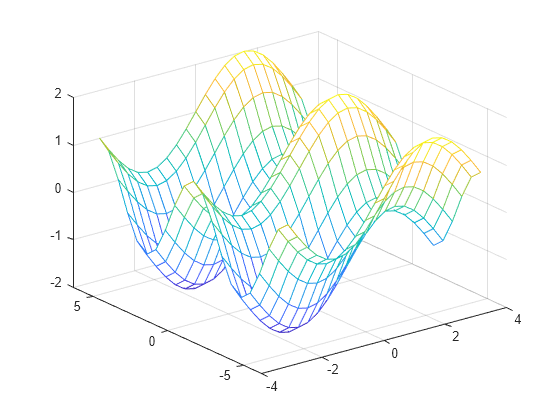
You can use the output from mygrid to create a mesh or surface plot:

z = sin(x) + cos(y);
mesh(x,y,z)

Arrays of Anonymous Functions

Although most MATLAB fundamental data types support multidimensional arrays, function handles must be scalars (single elements). However, you can store multiple function handles using a cell array or structure array. The most common approach is to use a cell array, such as

f = {@(x)x.^2;
     @(y)y+10;
     @(x,y)x.^2+y+10};

When you create the cell array, keep in mind

that MATLAB interprets spaces as column separators.

Either omit spaces from expressions, as shown in the previous code,

or enclose expressions in parentheses, such as

f = {@(x) (x.^2);
     @(y) (y + 10);
     @(x,y) (x.^2 + y + 10)};

Access the contents of a cell using curly braces.

For example, f{1} returns the first function handle. To execute the function, pass input values in parentheses after the curly braces:

x = 1;
y = 10;

f{1}(x)
f{2}(y)
f{3}(x,y)

ans =
     1

ans =
    20

ans =
    21